This document is a simple step-by-step introduction to the Equation Editor and related advanced functions of the Java version of SimForest. It contains a step-by-step example that will walk you through creating a simple new equation and assigning it to a new Tree Table parameter, which can then be graphed or used in other equations.
You will find some background information along the way, in paragraphs labeled Explanation and set in different type from the instructions. Feel free to skip these if you're following the example; come back and read them later if you're interested in more detailed, conceptual explanations of the steps you took.
Below the step-by-step example is a piece-by-piece description of the Equation Editor window. You may want to refer to this section if you are unsure about what part of the window the instructions are discussing.
In this example we will create an equation to compute the basal area of the trees in the simulation. This is simply the area of a slice through the tree's trunk at the same point where the diameter is measured. Assuming the trunk is perfectly circular, this will be equal to pi times the square of the radius (half the diameter).
Following these instructions, first, you will add the new equation to the list. Next, you will build it in the Equation Editor. After that, you will assign the equation to a new Tree Table parameter that you will create. Then, you will be able to graph the trees' Basal Area as they grow in the simulation.
Bring the Equation List window to the front by selecting it from the Window menu (in any open window). Then choose "New" from the "Equation" menu to create the new equation, and enter an appropriate name (like "Basal Area") in the resulting dialog box.
Once you click "OK", the new, empty Basal Area equation will be at the bottom of the Equation List. Double-click the new equation to open it in the Equation Editor.
At this point, the equation is empty: it doesn't contain any functions or constant values from which to compute its value. You are going to build the equation for Basal Area using the editor. While these instructions may seem wordy and complex to read, the tasks being described are actually fairly easy – once you are able to follow the first few steps, it should be relatively simple to build the whole equation.
Remember, this equation is going to be (3.14 * ((diameter / 2) ^ 2)), where * means multiplication, / means division, ^ means raising to a given power (i.e., N ^ 2 means N squared), and diameter is the current diameter of the tree in question.
Since the equation editor's representation of equation works from the outside inward to the more deeply nested parts of the equation, we will start with the outermost function, which is multiplication (pi times the square of the radius).
Explanation: You can see that this is the outermost function because it is the only one within the outermost set of parentheses. Each time we go deeper into the equation, this corresponds to removing one more set of parentheses (assuming that the text form of the equation uses parentheses around every operation, as I have done above).
Select the equation's name in the Equation panel (the large upper-right panel which displays the current form of the equation you're editing). Then select "Product" (under "Math") in the Tools panel on the left; this is the multiplication operation, which you are adding first. Double-click "Product" or click the "Add as Child" button in the button bar to add the multiplication operator to this equation.
Now you will add the arguments to this multiplication. The first argument is 3.14, or pi (you can use more digits if you want to be very precise). In the Equation panel, select the * representing the outer multiplication. Then select "Number" (under "Constants") in the Tools panel, and double-click it (or click "Add as Child") to add a new numeric constant to the multiplication. The constant will initially be 0 by default. Select the 0 in the Equation panel, and double-click it or click the "Edit Constant" button to edit its value. Type "3.14" in the resulting dialog and then click "OK" to make the change.
The multiplication's second argument is the square of the tree's radius, ((diameter / 2) ^ 2). This is a "Power" operation – the outermost function is the squaring of the radius, represented by ^. So select the * again in the Equation panel, and select "Power" (under "Math") in the Tools panel. Again, double-click "Power" (or click the "Add as Child" button) to add the square as an argument to the multiplication. The power, ^, will be entered before (above) the 3.14 that you added earlier; since order doesn't matter in multiplication, this is okay, but you can change the order by selecting the ^ and clicking the "Move Down" button (the down arrow) in the button bar.
Now you need to add the arguments to the ^ function, which raises its first argument to the power specified by its second argument. The first argument will be the tree's radius, (diameter / 2), and the second will be 2.
To add the first argument, notice that its outermost function (the only one left now that we've worked this far inward) is /, representing division. Select the ^ in the Equation panel, and select "Quotient" (under "Math") in the Tools panel; then, once again, double-click "Quotient" to add it as the square's first argument. Now you have the choice of completing the square before adding the arguments to the division, or building the division before adding the second argument to the ^ function.
To avoid confusion, let's complete the outer square first, by adding a 2 as its second argument. Select the ^ again in the Equation panel, and select "Number" (under "Constants") in the Tools panel; then double-click "Number" to add it as the square's second argument. The number constant will be 0 by default; double-click it in the Equation panel and enter "2" in the resulting dialog, then click "OK" to change its value to 2.
But, before you proceed, notice – the 2 was entered before (above) the / division in the editor, and order does matter here (we don't want to raise 2 to the power of the tree's radius). So select the 2 in the Equation panel and click the "Move Down" button (labeled by a downward-pointing arrow) to place the 2 below the division.
Now all that's left is to complete the division that represent's the tree's radius, (diameter / 2). This operation has two arguments; the first is the tree's diameter and the second is 2. You have probably noticed by now that the editor adds new arguments before the ones that are already in place, so let's add the 2 (the second argument) first this time, and then add the diameter. Select the / in the Equation panel, and double-click "Number" (below "Constants") in the Tools panel to add a new numeric constant to the equation; then double-click the number, which will be 0 by default, and change it to 2.
The only remaining thing to add is the tree's diameter, which we are dividing by 2 to provide its radius. Select the / again in the Equation panel. Then scroll down to the "Equations" section of the Tools panel and select the "Diameter" equation. Double-click "Diameter" to add it as an argument to the division.
Explanation: Notice that there are two places that it might seem reasonable to find the tree's current diameter: the Diameter equation, and the diameter column (parameter) in the Tree Table, which holds the result of evaluating the Diameter equation each year. In this situation you will almost always want to use the equation's value, not the table's – the number your equation gets from the table is last year's value, but the value of the equation is the current one.
Now the equation is complete!
To be sure you have built the equation correctly, select its name, which is the topmost and leftmost item in the Equation panel; then inspect the equation's text form in the bottom part of the Equation panel, and make sure it corresponds to the equation you had in mind.
When you are done inspecting the equation, close the Equation Editor window. Be sure to choose "Keep Changes" to preserve the new equation you have just constructed.
Now that you have constructed an equation that computes a tree's basal area, you will want to store its value in a table parameter in order to watch it change over time (and in order to graph it).
Explanation: In some circumstances, you might not want to store an equation's result in one of the simulation's tables. Some equations only exist in order to provide their values to other equations (like the "Nitrogen Factor", "Light Factor", and other equations, which are multiplied together by other equations). Some equations do not need to be evaluated in all circumstances (like the "Light Factor (shade-tolerant)" equation, which is only computed for trees of shade-tolerant species). In these cases, it does not make sense to store the equations' values in a table every year.
Bring the Tree Table window to the front by selecting it from the Window menu. Click the "New Parameter" button, then enter an appropriate name for the new parameter (like "ba") and click "OK" to create the new parameter. You've now created a new parameter, a new column in the table, with a cell for every tree. (You might have to resize the Tree Table window to bring the new column into view.)
But all those empty cells won't hold any value until you either type a value into them by hand, or assign an equation to the new parameter. In this case, you want the parameter to be dynamic (you want it to change every year according to the simulation), so it doesn't make sense to enter values by hand. You want to set the parameter from the equation you just created. Highlight the parameter's column by clicking in any cell in that column. Then go to the "Parameter" menu and select "Set from Equation". Choose the Basal Area equation that you just created, and click "OK". Now the parameter will be updated every year with the equation's value. Go ahead and try it out, if you want, by running the simulation for a year or two and examining the new values in the table.
Explanation: We chose to put the new parameter in the Tree Table, not the Species Table or the Site Table, because Basal Area is a property of each individual tree. It wouldn't make sense – in fact, the simulation wouldn't be able to compute the Basal Area equation's value – if you put it in the Species Table or the Site Table. In general:
Now that you have assigned the Basal Area equation to a parameter in the Tree table, you can examine the basal area of the simulation's trees using the graphing window. First, run the simulation for a few years to generate some data; then pause the simulation so that the program will respond more quickly.
From the Window menu, select "New Graph". This will create a new Graph window. You can have many Graph windows open at once to examine different values; the graphs will be updated automatically after each year in the simulation. (This may cause the simulation to run more slowly.)
By default, he Graph window shows a scatterplot of tree height (on the Y-axis) vs. tree age (on the X-axis), with each point in the graph representing an individual tree in the simulation. You can easily change this graph to show basal area vs. age instead by selecting the new parameter you just created in the Y-axis parameter popup menu (which is now showing "height").
Next, try graphing basal area vs. time, using either the stacking-area graph or the line graph: choose "Time (line)" or "Time (stacking)" from the X-axis graph type popup menu, in the top center. This graph automatically aggregates values by species, so you are seeing the total basal area of each species at each year over the course of the simulation. Notice that the lines and areas in this graph, like the points in the scatterplot, are colored to correspond to the species' colors in the main simulation window. You can change these colors in the main simulation window if you like.
Congratulations! You have completed the example. Feel free to experiment further – if you are worried about messing things up as you experiment, just save your equation set and your Tree Table (and/or Species and Site Tables) and then proceed. You can always restore the simulation from your saved files if you don't like the changes you've made.
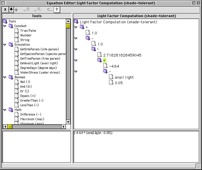
Here is an example of an Equation Editor window. You can have any number of Equation Editors open at once, showing different equations. You can open an Equation Editor by double-clicking an equation in the Equation List window (or double-clicking it in the Editor where it appears in another equation).
Apart from the menus, which are not shown in this illustration, the Equation Editor has the following functional components (we'll be referring to these in the step-by-step example):
[ Return to SimForest home page ]